Structure and parameterization
The "Eclipse" LSTM model is designed to predict cyclical patterns in Bitcoin markets using time-series data. The model architecture and its parameters have been carefully configured to ensure robustness and reliability in capturing temporal dependencies and nonlinear relationships. Below is a detailed explanation of its structure and parameterization:
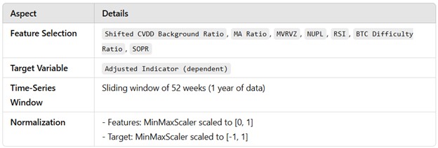
Input Data
In the development of the Eclipse indicator, a 52-week sliding window was selected as the optimal timeframe for modeling. This choice allows the model to capture a full year of weekly data, effectively incorporating seasonal trends and annual cycles that are critical in Bitcoin's market behavior. The 52-week window strikes an ideal balance between preserving sufficient historical context to identify long-term patterns and maintaining the responsiveness needed to reflect recent market dynamics.
Extensive testing was conducted with various window lengths, ranging from shorter to longer periods. These experiments revealed that shorter windows lacked the necessary context for detecting longer-term cycles, while longer windows introduced excessive noise, diminishing the model's ability to adapt to recent data. The 52-week window consistently produced the best performance and accuracy, making it the most effective choice for predicting cyclical tops and bottoms in Bitcoin’s market trends.
Model Architecture
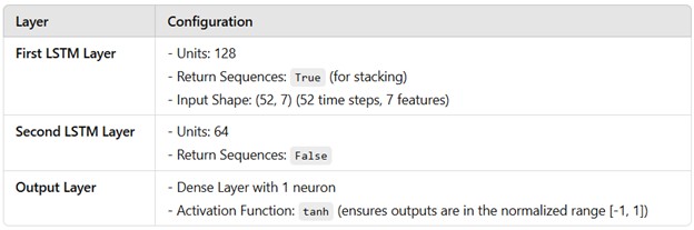
The use of 128 units provides a robust capacity for learning complex sequential patterns and relationships in the data. A higher number of units allows the model to capture subtle long-term dependencies and ensures that sufficient representational power is available for the feature-rich input.
Setting return_sequences=True is necessary to pass the entire sequence of hidden states to the next LSTM layer. This facilitates stacking multiple LSTM layers, enabling the model to learn hierarchical temporal features and improving its ability to detect multi-scale patterns in the data.
This shape reflects the model's input: 52 time steps (representing one year of weekly data) and 7 features (the selected independent variables). This configuration allows the model to effectively analyze relationships between features across the entire sliding window. A reduced number of units (64 compared to the first layer's 128) helps to distill and compress the information learned in the previous layer. This reduction minimizes overfitting while retaining critical temporal dependencies, enabling the model to focus on the most relevant patterns for prediction.
With return_sequences=False, this layer outputs only the final hidden state rather than the full sequence. This is appropriate for downstream dense layers that require a fixed-size input, such as the output layer used in this model. The dense layer consists of a single neuron, which produces the final prediction for the dependent variable. This ensures a one-to-one correspondence with the target output.
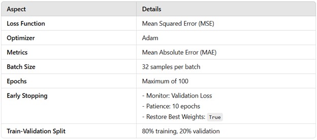
Training Configuration
A batch size of 32 balances computational efficiency and model performance, with a maximum of 100 epochs. However, Early Stopping halts training if the validation loss does not improve for 10 consecutive epochs, restoring the best weights to prevent overfitting. The data is split into 80% training and 20% validation, ensuring the model is evaluated effectively while being trained on a substantial portion of the data.